This is a bilingual snapshot page saved by the user at 2025-4-4 23:43 for https://www.yuque.com/yuqueyonghucrjh2o/ge8ik0/ggfl86mi3c8qarbd, provided with bilingual support by Immersive Translate. Learn how to save?
  💡 Get started quickly

  Building a Large Model Knowledge System from 0 (1): What is a Model?

  As is customary, conclusions come first
  What is this article going to discuss?
AI technology, represented by large models, has been unprecedentedly prosperous in the past two years. We believe that in such a context, it is necessary to start learning from the most basic concepts, and gradually establish a relatively complete knowledge system in order to understand the subsequent new concepts, new technologies, and new products. Therefore, this article is written to discuss the most basic concepts in the knowledge system of large models, and to pave the way for the subsequent articles in this series.

  How do you discuss this?
For the construction of a large model knowledge system, I think we need to understand the following issues first:
(1) Regardless of whether it is a large model or a small model, can you first explain what a model is?
(2) How exactly is the model trained with data, so that the trained model can be used to solve practical problems?
I will use a practical problem of predicting milk tea sales as a starting point, design and manually train a simplest model, and discuss the above two core questions step by step along the way.

  What are the core conclusions of these questions?
A model is essentially a mathematical formula, or more precisely, a function. Training a model is the process of using data to continuously update model parameters through a backpropagation algorithm to fit existing data. And because the trained model fits the existing data, we believe that it has mastered the statistical rules of the existing data, and then we can use this model (this law) to predict unknown situations.

"Dating an AI is like going on a 100-date date: it writes down everything you say as a cheat sheet and ends up with a love brain that understands you"
  —Epigraph

  Hand rub a milk tea sales prediction algorithm
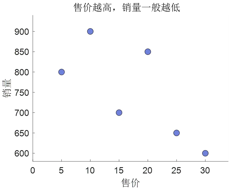
Let's say you work in a bubble tea shop, and the selling prices and sales of the 6 types of milk teas that have been on sale recently are as follows

  selling price
  Sales
  Milk tea 1
30
600
  Milk tea 2
25
650
  Milk tea 3
20
850
  Milk tea 4
15
700
  Milk tea 5
10
900
  Milk Tea 6
5
800
One day, the boss asked you, if a new milk tea is launched at this time, if it is priced at 35 without considering other factors, how much should it sell? In other words, if the selling price is set at 35, how much do you predict to sell?

Damn, the price of 35 is not within the scope of the existing data at all, how can this be done?

Of course, we don't want to make predictions out of thin air, but to make predictions that are most in line with the current data laws based on the existing data, otherwise the boss will be dumb if we ask one more why. Let's take a look at the data first, and it is not difficult to find that the higher the selling price, the lower the sales volume.
900
850
800
  Xinjiang residence
750
700
650
009
20
5
15
  selling price
image.png

Imagine, if there is a mathematical formula that can directly tell us how much the specific sales volume corresponding to different selling prices are, then the sales volume when the predicted selling price is 35 is not a bag to pick up things, hand to catch, hand to pinch?

But how do you find this mathematical formula? If we look closely at the graph above, we can see the selling price as the independent variable and the sales volume as the dependent variable, and the dependent variable decreases with the increase of the independent variable, which can be completely used as a function that we learned in the second grade of junior high school
  to describe, where the independent variables
  is the selling price, the dependent variable
  for sales,
are the two parameters in this formula for which specific values have not yet been determined. Once we can be sure
  The specific values are put again
  Substituting this formula into this formula gives you the predicted sales volume at a price of 35.

  At this point, the question of forecasting sales was translated into certainty
In other words, we build a mathematical model for predicting the sales of milk tea:


Wait...... Model? Parameter? Forecast? Could it be that what kind of large model do you usually hear, and hundreds of millions of parameters refer to this?

That's right! A large model is essentially a mathematical formula with an extremely complex form and an extremely large number of parameters. And the so-called forecast, just like the sales volume after we give the selling price, is just given a specific input and then calculated according to the formula.

  This is training
  Back to the question now: how to be sure
  What about the specific values?

  To recap, the image of a primary function is a straight line,
  Adjust the inclination of the line and the distance from the origin of the coordinate system, respectively
90%
x
y
y=2x+3
y=kx+b中,k越大,直线倾斜程度越大
 
3
y=kx+b中,b越大,直线距离原点越远
y=4x+3
x
y
x
y
x
y
y=2x+3
 
6
y=2x+6
所以我们要调整
的值,最好让整条直线能不偏不倚的贯穿这堆数据所围成的区域。换句话说,我们期望这条直线能最好的拟合当前的数据。

100%

但我们从哪个值开始尝试和调整呢?此外,调整之后我们怎么知道这算不算“最好的拟合”呢?

从哪个值开始尝试这个问题,实在不行就先猜一个呗。没错,就是猜!先上线再迭代!即便是第一个做出大模型的人在一开始确定参数的时候也是靠猜,只不过是有技巧的猜。

比如在我们这个例子当中考虑到销量随售价的增加而降低,即二者是负相关,所以
肯定得猜成负数才合理。且从奶茶1售价30销量600,奶茶2售价25销量650来看,售价每增加1,销量就减少10,所以我们先盲猜成-10(当然,这里选其他奶茶来猜也可以)。

的值看上图中直线与
轴的交点先盲猜成1000吧,于是我们得到了模型v1.0:
,同样,画出来先看看效果。
100%
这效果怎么说呢......大方向是对的,但肯定拟合得不算好。

至于怎么样算“最好的拟合”,我们可以这样定义:对于已知售价和销量的6款奶茶,我们先输入每款的售价,再通过模型得到每款的预测销量,然后计算预测销量与实际销量之间差值平方的一半作为模型对一款奶茶销量的拟合误差(之所以要用差值平方的一半而不用差值本身是因为这样做有有良好的数学特性)。若用
来表示拟合误差的话,
的表达式即为
,其中
即为我们通过模型得到的预测销量,
为奶茶的真实销量。然后我们把所有奶茶的拟合误差平均值作为模型对整个数据集的总拟合误差,只要我们不断调整
的具体数值能使得这个总拟合误差最小,此时便可认为是“最好的拟合”。

举例来说,现在我们的模型为
,第一款奶茶售价30,因此我们输入
得到输出的预测销量为700,与实际销量600差值平方的一半为
,也就是5000,第二款售价25,输入公式后得到输出的预测销量750,与实际650的销量差值平方的一半也为5000......以此类推可以得到第三至第六款奶茶的拟合误差分别为1250,11250,0,11250。最后对6个误差值求平均得到模型v1.0的总拟合误差为5625。

那我们应该怎样调整
使得总拟合误差最小的呢?这就不得不提到大名鼎鼎的“反向传播”算法了。既然有反向传播,那自然也有正向传播(实际上叫前向传播),我们先介绍前向传播。

所谓前向传播其实就是给定输入数据后通过模型得到输出结果的过程。例如对于我们当前的模型
,给定第一款奶茶的售价30,我们通过模型计算得到它的预测销量为
,这就完成了一次前向传播。

而反向传播则是根据拟合误差反向计算出模型中每个参数对这个误差“贡献度”的过程,其中涉及通过误差公式对模型参数求偏导数的数学运算,我们这里简单介绍一下。
(此部分无法理解不影响后续的阅读,总之就是我们有数学方法求得模型中每个参数对误差的贡献度)
之前提到,每款奶茶的拟合误差计算公式为
,而其中
,因此误差
对模型参数
的偏导即等于
的偏导乘以
的偏导。
对模型参数
的偏导即等于
的偏导乘以
的偏导。也就是:


比如还是第一款奶茶,模型对它销量的拟合误差为5000,这个误差对
求偏导后的结果分别为3000和100,这两个数可以粗暴解读为
这件事为拟合误差贡献了3000份力,而
贡献了100份力,二者一共贡献了3100份力导致了5000的误差。所以我们让
减去各自贡献的这份力就可以一定程度上减小拟合误差。只不过在减的时候我们希望“步子慢一点”,毕竟这只是第一款奶茶,咱之后还有5款奶茶要考虑,所以只减去3000和100的万分之一,也就是0.3和0.01即可,由此得到了更新后的参数
,此时我们得到了模型v1.1:


同样,我们用第二款奶茶的数据重复以上过程:
1输入第二款奶茶的售价
并利用模型v1.1
做前向传播得到预测销量742.49
2计算模型对第二款奶茶的拟合误差为4277.20,用其对
求偏导,得到二者为此误差的贡献度分别为2312.25和92.49
3用当前的
减去其各自贡献值的万分之一,得到
进而得到模型v1.2:


我们继续重复此过程直到6个数据点都已被用于反向传播调整参数,于是得到了模型v2.0:
,该模型对6个数据的总拟合误差为4847,比模型v1.0的5625低了很多。

把模型v1.0和2.0一起画出来对比下看看
100%
嗯~~不错,模型v2.0确实比1.0好一些,但是距离理想的拟合效果还是有一定差距。

到此,我们通过已有的数据来对模型的参数进行了一轮调整,这个过程就叫做训练,也可以叫做学习。总之就是调整模型的参数让它和已有的数据越来越拟合。

菜,就多练
但现在一轮训练下来模型的拟合效果还不够好,咋办呢?还能咋办,菜就多练呗。继续用已有的数据进行第二轮,第三轮训练......直到再怎么训练也不能显著降低模型误差时就可以结束了。

模型在训练前,以及1轮、5轮、15轮、20轮训练后的图像和误差如下图所示(其中模型v15.0与模型v20.0几乎重合):
100%
显然,同样是5轮训练,从模型v10.0到v15.0误差降低了17,但从v15.0到20.0就只降低了2。这说明从模型v20.0开始,再多的训练也不怎么能降低模型误差了,所以我们停止训练,直接取模型v20.0的参数
作为最终训练结果。

回到一开始的问题,老板问奶茶售价定为35,它预计的销量为多少呢?有了模型不难算出
,四舍五入一下得到我们的预测销量536。

复盘一下,我们学到了什么?

所谓数学建模就是将实际问题转化为数学问题,然后用数学工具去解决它。我们将预测奶茶销量的实际问题转化为了确定一次函数两个参数值的数学问题,并通过求偏导这一数学工具不断的优化参数值以求最好的拟合已有数据,最终确定参数值后输入售价得到了预测销量。

所谓模型,本质就是一套数学公式。无论大模型还是小模型,其本质都是一套数学公式,或者说函数。在预测奶茶销量这件事中,我们选取了只含两个参数的一次函数作为模型来完成预测工作。而大模型的的公式极复杂,参数量极多,以至于它可以先将我们输入的人话转化为可运算的数字,进行计算后输出另一句人话,从而完成与人对话这种神奇的事情。

所谓训练(或者学习),就是用数据通过反向传播算法不断调整模型中的参数。我们根据已有数据的分布特点猜了两个数作为模型参数的初始值,然后把已有数据一个又一个,一轮又一轮的送入模型中做前向传播和反向传播来调整参数,让模型更好的拟合已有数据。直到我们发现进行更多的训练也不能显著降低模型的误差后便停止训练。对于我们这样只有两个参数的模型都进行了20轮训练,可想而知拥有几十上百亿参数的大模型要进行多少训练,消耗多少算力。

欢迎来到1986
以反向传播算法为核心的模型训练机制出自1986年的文章《Learning Representations by Back - Propagating Errors》。到此,恭喜你对大模型知识的理解来到了1986年。此时距离DeepSeek-R1发布还有39年。

AI Heroes
模型之所以能被训练是因为反向传播算法让其能根据已有数据不断调整参数以进行更好的拟合。反向传播算法的代表作是 David E. Rumelhart、Geoffrey E. Hinton Ronald J. Williams 于 1986 年发表在《Nature》上的论文《Learning Representations by Back - Propagating Errors》。尽管在这之前也有类似的方法被提出,但此文将反向传播算法应用于多层神经网络,并证明了其在机器学习中的有效性,对现代神经网络和深度学习领域产生了深远的影响。

其中,Rumelhart于2011年逝世,享年70岁。 Williams于2024年逝世,享年79岁。Hinton于2024年获得诺贝尔物理学奖以表彰其为机器学习领域作出的基础性发现和发明。

高中时的 Hinton 就对人脑机制产生了浓厚兴趣,在大学期间,他虽然不断更换专业,但一直围绕着探索人脑神经元如何连接并工作的奥秘,这一兴趣促使他在读博期间选择了神经网络作为研究方向。现在如火如荼的神经网络在当时并不是一个被看好的方向,甚至在1978年Hinton博士毕业的时候,其博士生导师也建议他之后能更换研究方向,但他依旧遵循自己对人脑工作机制的探索欲望而在这个方向行走着,一路成果颇丰,桃李满天。

2012年,他与学生Alex Krizhevsky, Ilya Sutskever所合作的AlexNet在当年的ImageNet大规模视觉识别挑战赛(ILSVRC)上以显著优势取得了冠军,开启了深度学习的新时代。其中 Ilya Sutskever 于2015 年加入了一家创业公司,作为CTO和联合创始人领导了大模型相关的研究工作,并于2023年底发布chatGPT开启了大模型时代。这家大名鼎鼎的创业公司名叫——OpenAI。

行文至此,谨以诺奖评辞致敬这位把神经网络从坟墓里挖出来的孤勇者。

“For foundational discoveries and inventions that enable machine learning with artificial neural networks”
image.png

Geoffrey E. Hinton, 2024 年于斯德哥尔摩举行的诺贝尔奖演讲上发表讲话


“他用物理的语言赋予机器自学的能力,让神经网络从理论玩具成长为重塑世界的智能引擎。”
——后记


如果有帮助,还望点个赞,谢谢~
image.png


以下是文中为易于理解而表述不严谨之处,不读不影响理解后续文章
比如还是第一款奶茶,模型对它销量的拟合误差为5000,这个误差对
求偏导后的结果分别为3000和100,这两个数可以粗暴解读为
这件事为拟合误差贡献了3000份力,而
贡献了100份力,二者一共贡献了3100份力导致了5000的误差
这里将误差函数对
的偏导数相加得到3100实际上是没有意义的,类似于将一个苹果和一头猪相加一样没有意义。


关于我:
计算机背景的C端产品经理
期望能用AI做些不一样的事情,有机会欢迎联系,期待与同频者相遇
a29d5628873165e71284c4fea8a8597.jpg


今天 23:32
141
IP 属地贵州
划词评论(0)
夜雨思晗
Ctrl + ⇧ + 7有序列表

  4738 words
Adblocker